Colormaps¶

ProPlot defines colormaps as color palettes that sample some continuous function between two end colors. Colormaps are generally used to encode data values on a pseudo-third dimension. They are are implemented with the LinearSegmentedColormap and PerceptuallyUniformColormap classes, which are subclassed from matplotlib.colors.LinearSegmentedColormap.

ProPlot adds several features to help you use colormaps effectively in your figures. This section documents the new registered colormaps, explains how to make and modify colormaps, and shows how to apply them to your plots.

Included colormaps¶

On import, ProPlot registers a few sample perceptually uniform colormaps, plus several colormaps from other online data viz projects. Use show_cmaps to generate a table of registered maps. The figure is broken down into the following sections:

“User” colormaps, i.e. colormaps saved to your ~/.proplot/cmaps folder. You make new colormaps and add them to this folder using the Colormap constructor function.
Matplotlib and seaborn original colormaps.
ProPlot original perceptually uniform colormaps.
The cmOcean colormaps, designed for oceanographic data but useful for everyone.
Fabio Crameri’s “scientific colour maps”.
Cynthia Brewer’s ColorBrewer colormaps, included with matplotlib by default.
Colormaps from the SciVisColor project. There are so many of these because they are intended to be merged into more complex colormaps.

ProPlot removes some default matplotlib colormaps with erratic color transitions.

Note

Colormap and color cycle identification is more flexible in ProPlot. The names are are case-insensitive (e.g., 'Viridis', 'viridis', and 'ViRiDiS' are equivalent), diverging colormap names can be specified in their “reversed” form (e.g., 'BuRd' is equivalent to 'RdBu_r'), and appending '_r' or '_s' to any colormap name will return a reversed or shifted version of the colormap or color cycle. See ColormapDatabase for more info.

[1]:

import proplot as pplt
fig, axs = pplt.show_cmaps()

Perceptually uniform colormaps¶

ProPlot’s custom colormaps are instances of the PerceptuallyUniformColormap class. These colormaps generate colors by interpolating between coordinates in any of the following three colorspaces:

HCL (a.k.a. CIE LChuv): A purely perceptually uniform colorspace, where colors are broken down into “hue” (color, range 0-360), “chroma” (saturation, range 0-100), and “luminance” (brightness, range 0-100). This space is difficult to work with due to impossible colors – colors that, when translated back from HCL to RGB, result in RGB channels greater than 1.
HPL (a.k.a. HPLuv): Hue and luminance are identical to HCL, but 100 saturation is set to the minimum maximum saturation across all hues for a given luminance. HPL restricts you to soft pastel colors, but is closer to HCL in terms of uniformity.
HSL (a.k.a. HSLuv): Hue and luminance are identical to HCL, but 100 saturation is set to the maximum saturation for a given hue and luminance. HSL gives you access to the entire RGB colorspace, but often results in sharp jumps in chroma.

The colorspace used by each PerceptuallyUniformColormap is set with the space keyword arg. To plot arbitrary cross-sections of these colorspaces, use show_colorspaces (the black regions represent impossible colors). To see how colormaps vary with respect to each channel, use show_channels. Some examples are shown below.

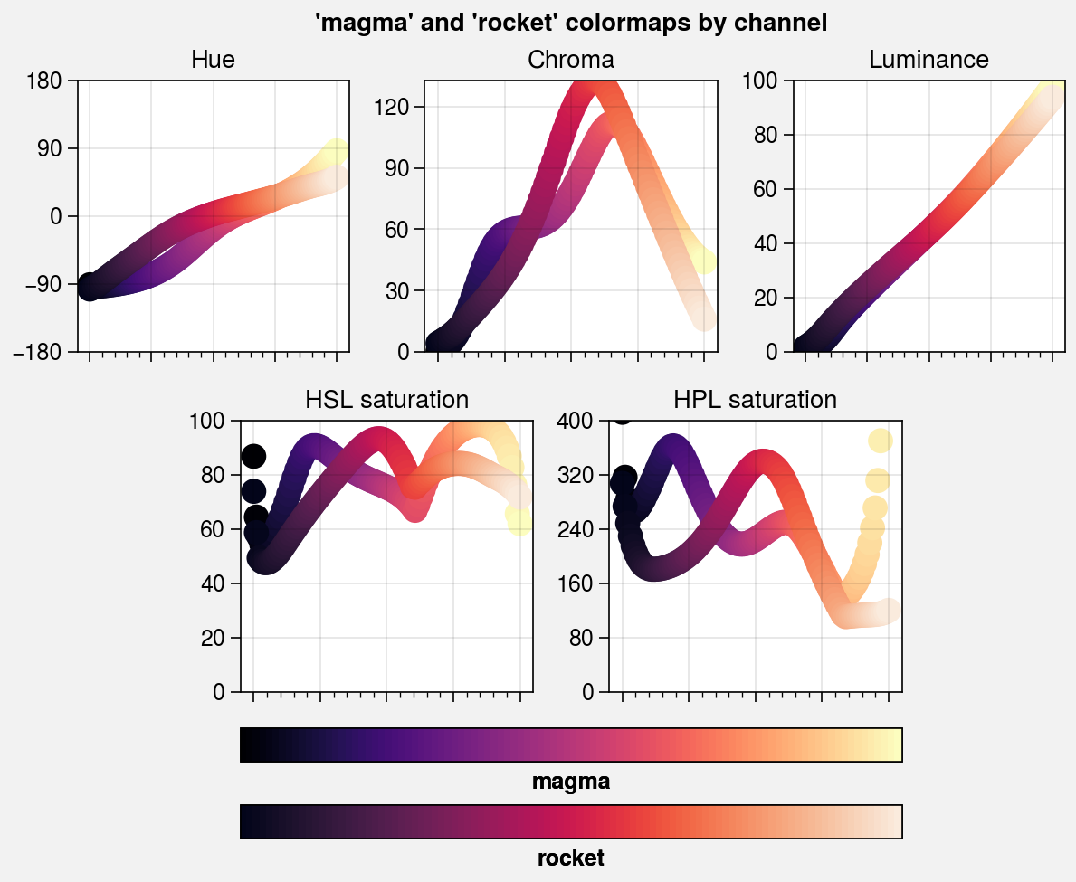
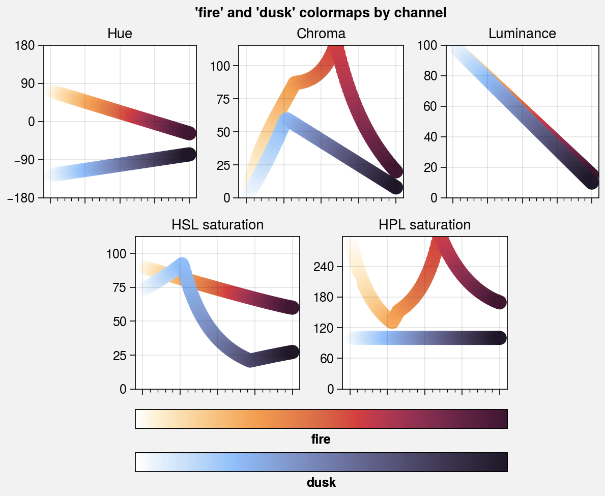
In theory, “uniform” colormaps should have straight lines in hue, chroma, and luminance (second figure, top row). In practice, this is difficult to accomplish due to impossible colors. Matplotlib and seaborn’s 'magma' and 'Rocket' colormaps are fairly linear with respect to hue and luminance, but not chroma. ProPlot’s 'Fire' is linear in hue, luminance, and HSL saturation (bottom left), while 'Dusk' is linear in hue, luminance, and HPL saturation (bottom right).

[2]:

# Colorspace demo
import proplot as pplt
fig, axs = pplt.show_colorspaces(refwidth=1.6, luminance=50)
fig, axs = pplt.show_colorspaces(refwidth=1.6, saturation=60)
fig, axs = pplt.show_colorspaces(refwidth=1.6, hue=0)

[3]:

# Compare colormaps
import proplot as pplt
for cmaps in (('magma', 'rocket'), ('fire', 'dusk')):
    fig, axs = pplt.show_channels(
        *cmaps, refwidth=1.5, minhue=-180, maxsat=400, rgb=False
    )

Making new colormaps¶

ProPlot doesn’t just include new colormaps – it provides tools for merging colormaps, modifying colormaps, making perceptually uniform colormaps from scratch, and saving the results for future use. For your convenience, most of these features can be accessed via the Colormap constructor function. Note that every plotting command that accepts a cmap keyword passes it through this function (see apply_cmap).

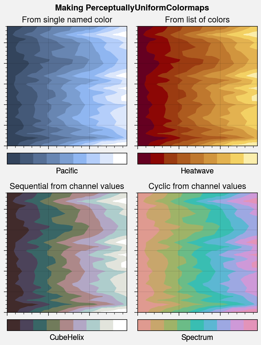
To make PerceptuallyUniformColormaps from scratch, you have the following three options:

Pass a color name, hex string, or RGB tuple to Colormap. This builds a monochromatic (single hue) colormap by calling the from_color static method. The colormap colors will vary from the specified color to pure white or some shade near white (see the fade keyword arg).
Pass a list of colors to Colormap. This calls the from_list static method, which linearly interpolates between each color in hue, saturation, and luminance.
Pass a dictionary to Colormap. This calls the from_hsl static method, which draws lines between channel values specified by the keyword arguments hue, saturation, and luminance. The values can be numbers, color strings, or lists thereof. Numbers indicate the channel value. For color strings, the channel value is inferred from the specified color. You can end any color string with '+N' or '-N' to offset the channel value by the number N.

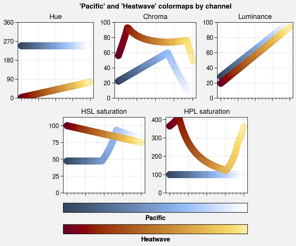
In the below example, we use all of these methods to make brand new PerceptuallyUniformColormaps in the 'hsl' and 'hpl' colorspaces.

[4]:

import proplot as pplt
import numpy as np
state = np.random.RandomState(51423)
data = state.rand(30, 30).cumsum(axis=1)

# Initialize figure
fig, axs = pplt.subplots(ncols=2, nrows=2, refwidth=2, span=0)
axs.format(
    xticklabels='none',
    yticklabels='none',
    suptitle='Making PerceptuallyUniformColormaps'
)

# Colormap from a color
# The trailing '_r' makes the colormap go dark-to-light instead of light-to-dark
cmap1 = pplt.Colormap('prussian blue_r', l=100, name='Pacific', space='hpl')
ax = axs[0]
ax.format(title='From single named color')
m = ax.contourf(data, cmap=cmap1)
ax.colorbar(m, loc='b', ticks='none', label=cmap1.name)

# Colormap from lists
cmap2 = pplt.Colormap(('maroon', 'light tan'), name='Heatwave')
ax = axs[1]
ax.format(title='From list of colors')
m = ax.contourf(data, cmap=cmap2)
ax.colorbar(m, loc='b', ticks='none', label=cmap2.name)

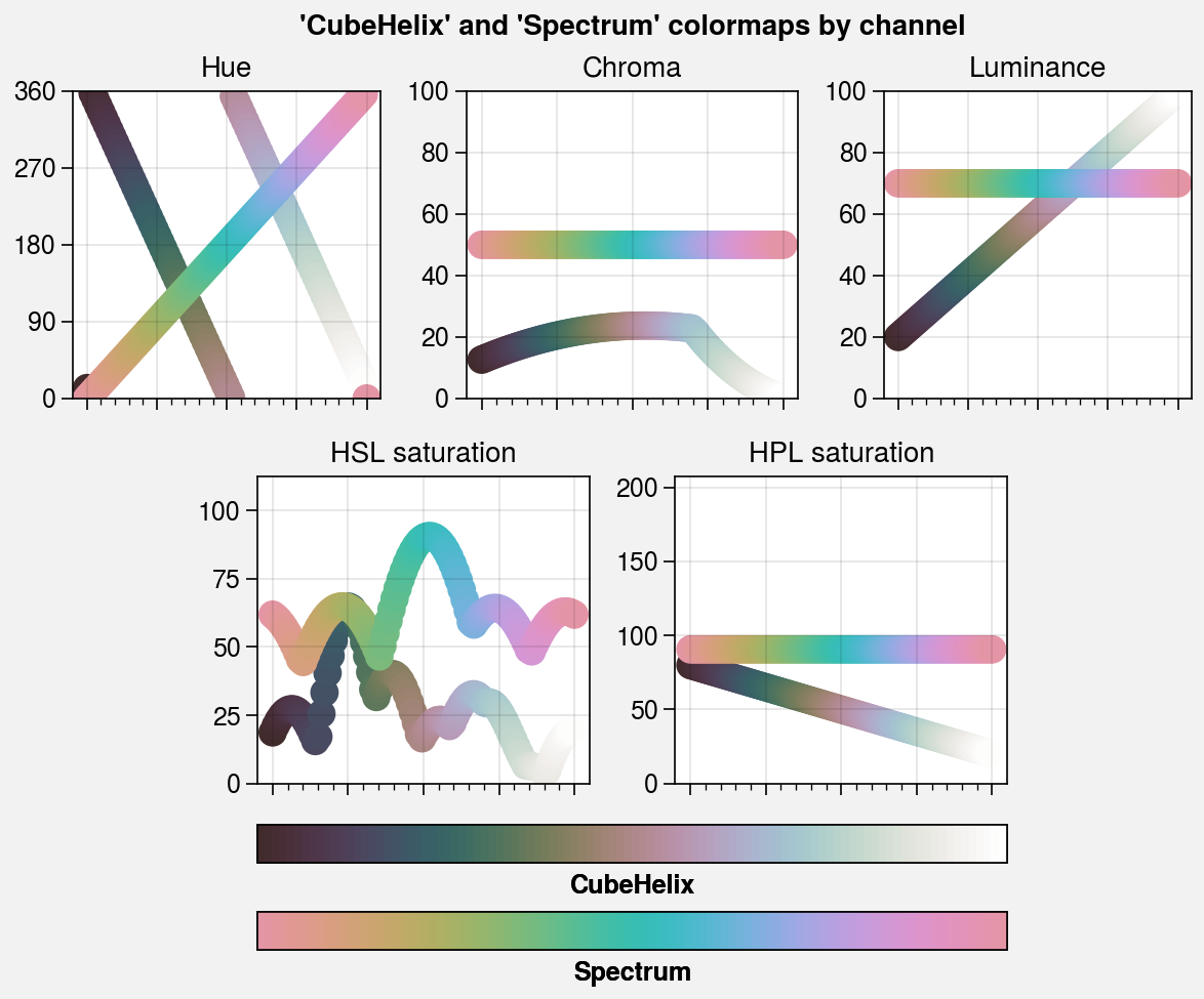
# Sequential colormap from channel values
cmap3 = pplt.Colormap(
    h=('red', 'red-720'), s=(80, 20), l=(20, 100), space='hpl', name='CubeHelix'
)
ax = axs[2]
ax.format(title='Sequential from channel values')
m = ax.contourf(data, cmap=cmap3)
ax.colorbar(m, loc='b', ticks='none', label=cmap3.name)

# Cyclic colormap from channel values
cmap4 = pplt.Colormap(
    h=(0, 360), c=50, l=70, space='hcl', cyclic=True, name='Spectrum'
)
ax = axs[3]
ax.format(title='Cyclic from channel values')
m = ax.contourf(data, cmap=cmap4)
ax.colorbar(m, loc='b', ticks='none', label=cmap4.name)

# Display the channels
fig, axs = pplt.show_channels(cmap1, cmap2, refwidth=1.5, rgb=False)
fig, axs = pplt.show_channels(cmap3, cmap4, refwidth=1.5, rgb=False)

Merging colormaps¶

To merge colormaps, simply pass multiple positional arguments to the Colormap constructor. This calls the append method. Each positional argument can be a colormap name, a colormap instance, or a special argument that generates a new colormap on-the-fly. This lets you create new diverging colormaps and segmented SciVisColor style colormaps right inside ProPlot. Segmented colormaps are often desirable for complex datasets with complex statistical distributions.

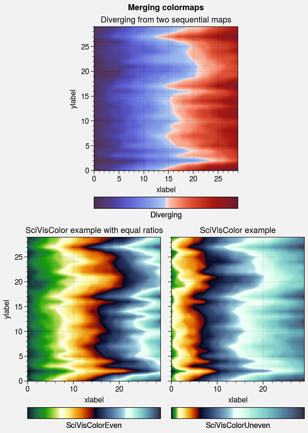
In the below example, we create a new divering colormap and reconstruct the colormap from this SciVisColor example. We also save the results for future use by passing save=True to Colormap.

[5]:

import proplot as pplt
import numpy as np
state = np.random.RandomState(51423)
data = state.rand(30, 30).cumsum(axis=1)

# Generate figure
fig, axs = pplt.subplots([[0, 1, 1, 0], [2, 2, 3, 3]], refwidth=2.4, span=False)
axs.format(
    xlabel='xlabel', ylabel='ylabel',
    suptitle='Merging colormaps'
)

# Diverging colormap example
title1 = 'Diverging from two sequential maps'
cmap1 = pplt.Colormap('Blues4_r', 'Reds3', name='Diverging', save=True)

# SciVisColor examples
title2 = 'SciVisColor example with equal ratios'
cmap2 = pplt.Colormap(
    'Greens1_r', 'Oranges1', 'Blues1_r', 'Blues6',
    name='SciVisColorEven', save=True
)
title3 = 'SciVisColor example'
cmap3 = pplt.Colormap(
    'Greens1_r', 'Oranges1', 'Blues1_r', 'Blues6',
    ratios=(1, 3, 5, 10), name='SciVisColorUneven', save=True
)

# Plot examples
for ax, cmap, title in zip(axs, (cmap1, cmap2, cmap3), (title1, title2, title3)):
    m = ax.contourf(data, cmap=cmap, levels=500)
    ax.colorbar(m, loc='b', locator='null', label=cmap.name)
    ax.format(title=title)

Saved colormap to '/home/docs/.proplot/cmaps/Diverging.json'.
Saved colormap to '/home/docs/.proplot/cmaps/SciVisColorEven.json'.
Saved colormap to '/home/docs/.proplot/cmaps/SciVisColorUneven.json'.

Modifying colormaps¶

ProPlot lets you create modified versions of existing colormaps using the Colormap constructor and the new LinearSegmentedColormap and ListedColormap classes, which are used to replace the native matplotlib colormap classes. They can be modified in the following ways:

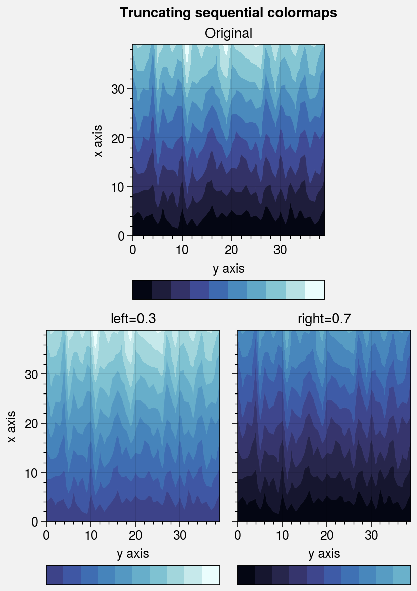
To remove colors from the left or right ends of a colormap, pass left or right to Colormap. This calls the truncate method, and can be useful when you want to use colormaps as color cycles and need to remove the “white” part so that your lines stand out against the background.
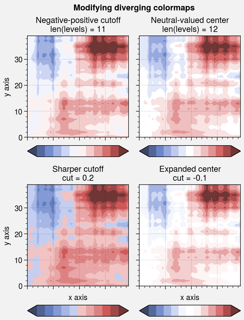
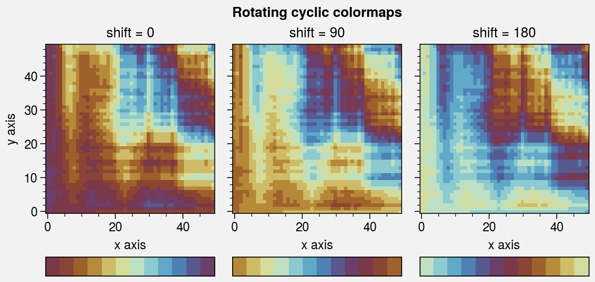
To modify the central colors of a diverging colormap, pass cut to Colormap. This calls the cut method, and can be used to create a sharper cutoff between negative and positive values or (when cut is negative) to expand the “neutral” region of the colormap.
To rotate a cyclic colormap, pass shift to Colormap. This calls the shifted method. ProPlot ensures the colors at the ends of “shifted” colormaps are distinct so that levels never blur together.
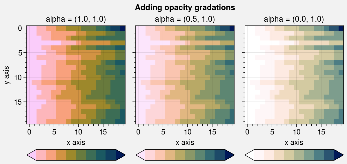
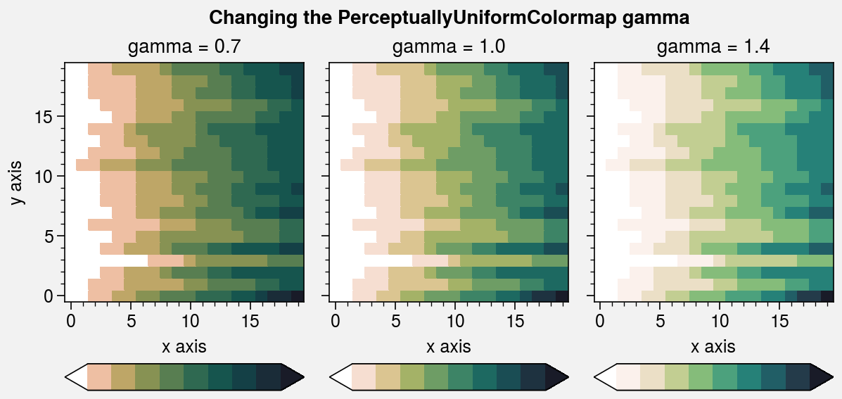
To change the opacity of a colormap or add an opacity gradation, pass alpha to Colormap. This calls the set_alpha method, and can be useful when layering filled contour or mesh elements.
To change the “gamma” of a PerceptuallyUniformColormap, pass gamma to Colormap. This calls the set_gamma method, and controls how the luminance and saturation channels vary between colormap segments. gamma > 1 emphasizes high luminance, low saturation colors, while gamma < 1 emphasizes low luminance, high saturation colors. This is similar to the effect of the HCL wizard “power” sliders.

[6]:

import proplot as pplt
import numpy as np
state = np.random.RandomState(51423)
data = state.rand(40, 40).cumsum(axis=0)

# Generate figure
fig, axs = pplt.subplots(
    [[0, 1, 1, 0], [2, 2, 3, 3]], refwidth=1.9, span=False,
)
axs.format(
    xlabel='y axis', ylabel='x axis',
    suptitle='Truncating sequential colormaps',
)

# Cutting left and right
cmap = 'Ice'
for ax, coord in zip(axs, (None, 0.3, 0.7)):
    if coord is None:
        title, cmap_kw = 'Original', {}
    elif coord < 0.5:
        title, cmap_kw = f'left={coord}', {'left': coord}
    else:
        title, cmap_kw = f'right={coord}', {'right': coord}
    ax.format(title=title)
    ax.contourf(
        data, cmap=cmap, cmap_kw=cmap_kw,
        colorbar='b', colorbar_kw={'locator': 'null'}
    )

[7]:

import proplot as pplt
import numpy as np
state = np.random.RandomState(51423)
data = (state.rand(40, 40) - 0.5).cumsum(axis=0).cumsum(axis=1)

# Generate figure
fig, axs = pplt.subplots(ncols=2, nrows=2, refwidth=1.7, span=False)
axs.format(
    xlabel='x axis', ylabel='y axis', xticklabels='none',
    suptitle='Modifying diverging colormaps',
)

# Cutting out central colors
levels = pplt.arange(-10, 10, 2)
for i, (ax, cut) in enumerate(zip(axs, (None, None, 0.2, -0.1))):
    levels = pplt.arange(-10, 10, 2)
    if i == 1 or i == 3:
        levels = pplt.edges(levels)
    if i < 2:
        title = 'Negative-positive cutoff' if i == 0 else 'Neutral-valued center'
        title = f'{title}\nlen(levels) = {len(levels)}'
    else:
        title = 'Sharper cutoff' if cut > 0 else 'Expanded center'
        title = f'{title}\ncut = {cut}'
    ax.format(title=title)
    m = ax.contourf(
        data, cmap='Div', cmap_kw={'cut': cut},
        extend='both', levels=levels,
        colorbar='b', colorbar_kw={'locator': 'null'},
    )

[8]:

import proplot as pplt
import numpy as np
state = np.random.RandomState(51423)
data = (state.rand(50, 50) - 0.48).cumsum(axis=0).cumsum(axis=1) % 30

# Rotating cyclic colormaps
fig, axs = pplt.subplots(ncols=3, refwidth=1.7, span=False)
for ax, shift in zip(axs, (0, 90, 180)):
    m = ax.pcolormesh(data, cmap='romaO', cmap_kw={'shift': shift}, levels=12)
    ax.format(
        xlabel='x axis', ylabel='y axis', title=f'shift = {shift}',
        suptitle='Rotating cyclic colormaps'
    )
    ax.colorbar(m, loc='b', locator='null')

[9]:

import proplot as pplt
import numpy as np
state = np.random.RandomState(51423)
data = state.rand(20, 20).cumsum(axis=1)

# Changing the colormap opacity
fig, axs = pplt.subplots(ncols=3, refwidth=1.7, span=False)
for ax, alpha in zip(axs, (1.0, 0.5, 0.0)):
    alpha = (alpha, 1.0)
    cmap = pplt.Colormap('batlow_r', alpha=alpha)
    m = ax.imshow(data, cmap=cmap, levels=10, extend='both')
    ax.colorbar(m, loc='b', locator='none')
    ax.format(
        title=f'alpha = {alpha}', xlabel='x axis', ylabel='y axis',
        suptitle='Adding opacity gradations'
    )

/tmp/ipykernel_3035/4264107422.py:12: ProPlotWarning: Using manual alpha-blending for 'batlow_r_copy' colorbar solids.
  ax.colorbar(m, loc='b', locator='none')
/tmp/ipykernel_3035/4264107422.py:12: ProPlotWarning: Using manual alpha-blending for 'batlow_r_copy' colorbar solids.
  ax.colorbar(m, loc='b', locator='none')

[10]:

import proplot as pplt
import numpy as np
state = np.random.RandomState(51423)
data = state.rand(20, 20).cumsum(axis=1)

# Changing the colormap gamma
fig, axs = pplt.subplots(ncols=3, refwidth=1.7, span=False)
for ax, gamma in zip(axs, (0.7, 1.0, 1.4)):
    cmap = pplt.Colormap('boreal', gamma=gamma)
    m = ax.pcolormesh(data, cmap=cmap, levels=10, extend='both')
    ax.colorbar(m, loc='b', locator='none')
    ax.format(
        title=f'gamma = {gamma}', xlabel='x axis', ylabel='y axis',
        suptitle='Changing the PerceptuallyUniformColormap gamma'
    )

Downloading colormaps¶

There are plenty of online interactive tools for generating perceptually uniform colormaps, including Chroma.js, HCLWizard, HCL picker, the CCC-tool, and SciVisColor.

To add colormaps downloaded from any of these sources, save the colormap data to a file in your ~/.proplot/cmaps folder and call register_cmaps (or restart your python session), or use from_file. The file name is used as the registered colormap name. See from_file for a table of valid file extensions.