Color cycles

ProPlot defines color cycles as color palettes comprising sets of distinct colors. Unlike colormaps, interpolation between these colors may not make sense. Color cycles are generally used with bar plots, line plots, and other distinct plot elements. ProPlot’s named color cycles are actually registered as ListedColormap instances so that they can be used with categorical data. Much more commonly, we build property cycles from the ListedColormap colors using the Cycle constructor function or by drawing samples from continuous colormaps.

ProPlot adds several features to help you use color cycles effectively in your figures. This section documents the new registered color cycles, explains how to make and modify colormaps, and shows how to apply them to your plots.

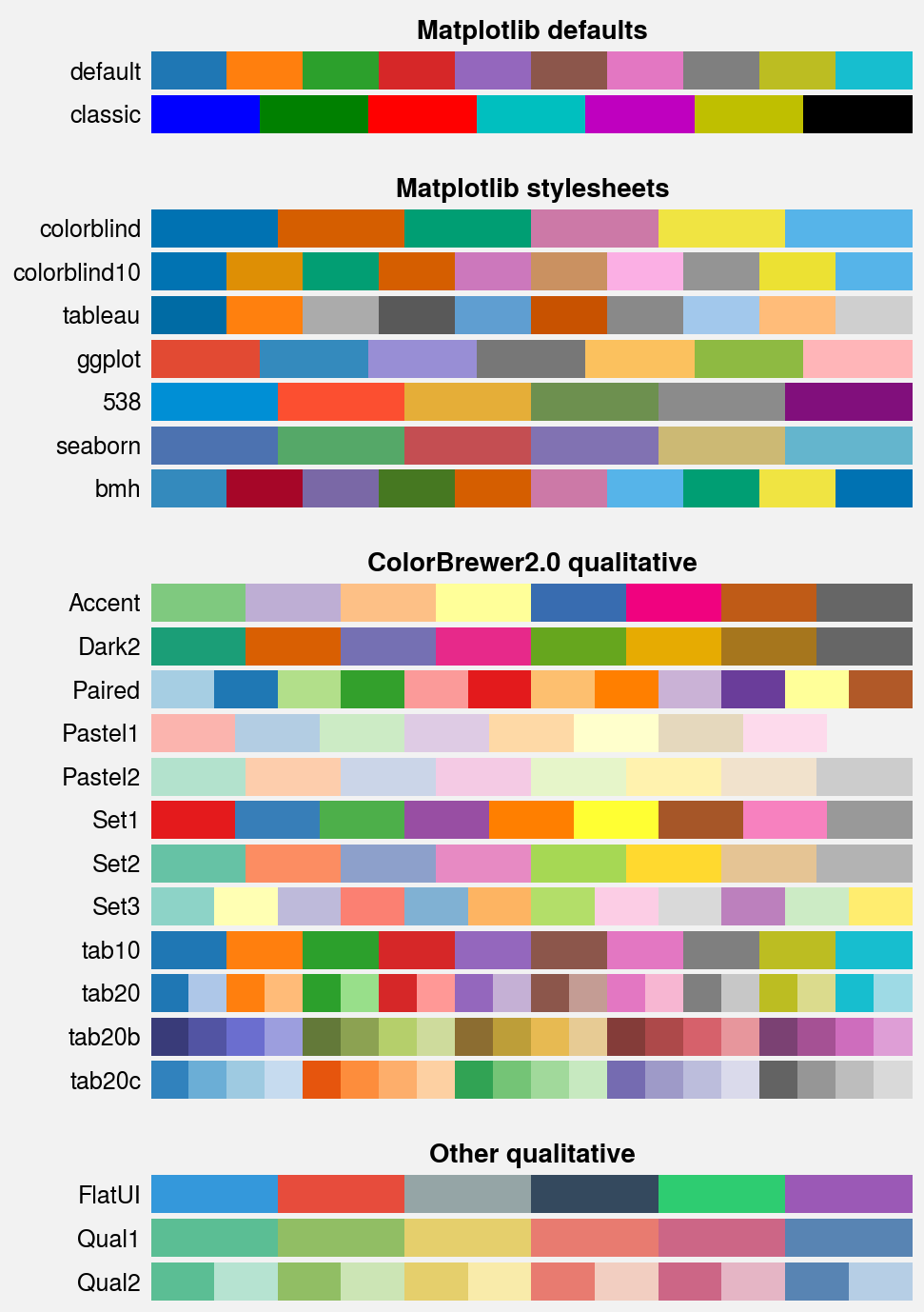
Included color cycles

Use show_cycles to generate a table of the color cycles registered by default and loaded from your ~/.proplot/cycles folder. You can make new color cycles and add them to this folder using the Cycle constructor function. To retrieve the list of colors associated with the color cycle, use Colors.

import proplot as pplt
fig, axs = pplt.show_cycles()

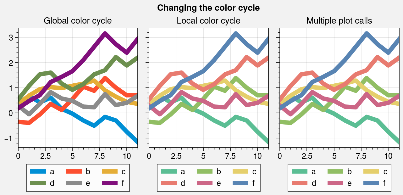
Changing the color cycle

Various plotting commands like plot and scatter now accept a cycle keyword arg, which is passed to the Cycle constructor function (see apply_cycle). To save your color cycle data and use it every time ProPlot is imported, simply pass save=True to Cycle. If you want to change the global property cycler, pass a name to the rc.cycle setting or pass the result of Cycle to the rc[‘axes.prop_cycle’] setting (see the configuration guide).

import proplot as pplt
import numpy as np

# Sample data
state = np.random.RandomState(51423)
data = (state.rand(12, 6) - 0.45).cumsum(axis=0)
kwargs = {'legend': 'b', 'labels': list('abcdef')}

# Figure
lw = 5
pplt.rc.cycle = '538'
fig, axs = pplt.subplots(ncols=3, refwidth=1.9)
axs.format(suptitle='Changing the color cycle')

# Modify the default color cycle
ax = axs[0]
ax.plot(data, lw=lw, **kwargs)
ax.format(title='Global color cycle')

# Pass the cycle to a plotting command
ax = axs[1]
ax.plot(data, cycle='qual1', lw=lw, **kwargs)
ax.format(title='Local color cycle')

# As above but draw each line individually
# Note that passing cycle=name to successive plot calls does
# not reset the cycle position if the cycle is unchanged
ax = axs[2]
labels = kwargs['labels']
for i in range(data.shape[1]):
    ax.plot(data[:, i], cycle='qual1', legend='b', label=labels[i], lw=lw)
ax.format(title='Multiple plot calls')

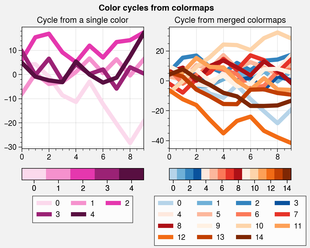
Making new color cycles

You can make new color cycles with the Cycle constructor function. One great way to make cycles is by sampling a colormap! Just pass the colormap name to Cycle, and optionally specify the number of samples you want to draw as the last positional argument (e.g., pplt.Cycle('Blues', 5)).

Positional arguments passed to Cycle are interpreted by the Colormap constructor, and the resulting colormap is sampled at discrete values. To exclude near-white colors on the end of a colormap, pass e.g. left=x to Cycle, or supply a plotting command with e.g. cycle_kw={'left': x}. See the colormaps section for details.

In the below example, several cycles are constructed from scratch, and the lines are referenced with colorbars and legends. Note that ProPlot allows you to generate colorbars from lists of artists.

import proplot as pplt
import numpy as np
fig, axs = pplt.subplots(ncols=2, share=0, refwidth=2)
state = np.random.RandomState(51423)
data = (20 * state.rand(10, 21) - 10).cumsum(axis=0)

# Cycle from on-the-fly monochromatic colormap
ax = axs[0]
lines = ax.plot(data[:, :5], cycle='plum', lw=5)
fig.colorbar(lines, loc='b', col=1, values=np.arange(0, len(lines)))
fig.legend(lines, loc='b', col=1, labels=np.arange(0, len(lines)))
ax.format(title='Cycle from a single color')

# Cycle from registered colormaps
ax = axs[1]
cycle = pplt.Cycle('blues', 'reds', 'oranges', 15, left=0.1)
lines = ax.plot(data[:, :15], cycle=cycle, lw=5)
fig.colorbar(lines, loc='b', col=2, values=np.arange(0, len(lines)), locator=2)
fig.legend(lines, loc='b', col=2, labels=np.arange(0, len(lines)), ncols=4)
ax.format(
    title='Cycle from merged colormaps',
    suptitle='Color cycles from colormaps'
)

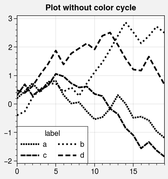
Cycles of other properties

Cycle can also generate cyclers that change properties other than color. Below, a single-color dash style cycler is constructed and applied to the axes locally. To apply it globally, simply use pplt.rc['axes.prop_cycle'] = cycle.

import proplot as pplt
import numpy as np
import pandas as pd

# Cycle that loops through 'dashes' Line2D property
cycle = pplt.Cycle(lw=2, dashes=[(1, 0.5), (1, 1.5), (3, 0.5), (3, 1.5)])

# Sample data
state = np.random.RandomState(51423)
data = (state.rand(20, 4) - 0.5).cumsum(axis=0)
data = pd.DataFrame(data, columns=pd.Index(['a', 'b', 'c', 'd'], name='label'))

# Plot data
fig, ax = pplt.subplots(refwidth=2.5)
ax.format(suptitle='Plot without color cycle')
obj = ax.plot(
    data, cycle=cycle, legend='ll',
    legend_kw={'ncols': 2, 'handlelength': 2.5}
)

Downloading color cycles

There are plenty of online interactive tools for generating and testing color cycles, including i want hue, coolers, and viz palette.

To add color cycles downloaded from any of these sources, save the cycle data to a file in your ~/.proplot/cycles folder and call register_cycles (or restart your python session), or use from_file. The file name is used as the registered cycle name. See from_file for a table of valid file extensions.