Subplots
A-b-c labels
ProPlot can be used to add “a-b-c” labels to subplots. This is possible
because subplots assigns unique numbers
to each subplot. If you passed an array to
subplots, the subplot numbers correspond to the numbers in
the array. If you used the ncols and nrows keyword arguments, the number
order is row-major by default but can be switched to column-major by passing
order='F' to subplots. The number order also determines the
subplot order in the SubplotsContainer returned by
subplots.
To turn on “a-b-c” labels, set rc.abc to True or pass
abc=True to format (see
the format command for details). To change the label
style, modify rc[‘abc.style’] or pass e.g. abcstyle='A.' to
format. You can also modify the “a-b-c” label
location, weight, and size with the rc[‘abc.loc’], rc[‘abc.weight’],
and rc[‘abc.size’] settings. Also note that if the an “a-b-c” label
and title are in the same position, they are automatically offset
away from each other.
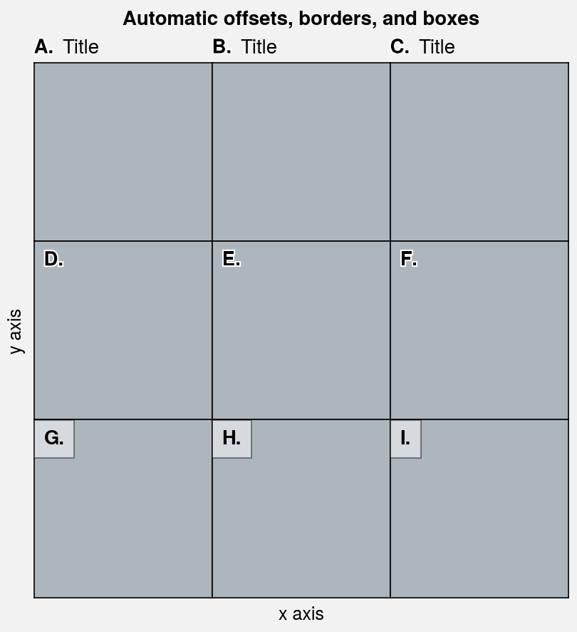
Note
“Inner” a-b-c labels and titles are surrounded with a white border when
rc[‘abc.border’] and rc[‘title.border’] are True (the default).
White boxes can be used instead by setting rc[‘abc.bbox’] and
rc[‘title.bbox’] to True. These options help labels stand
out against plotted content. These “borders” and “boxes”
can also be used by passing border=True or bbox=True to
text, which ProPlot wraps with
text_extras. See the plotting sections
for details on wrapper functions.
[1]:
import proplot as pplt
fig, axs = pplt.subplots(ncols=3, nrows=3, space=0, refwidth='10em')
axs.format(
    abc=True, abcloc='ul', abcstyle='A.',
    xticks='null', yticks='null', facecolor='gray5',
    xlabel='x axis', ylabel='y axis',
    suptitle='Automatic offsets, borders, and boxes',
)
axs[:3].format(abcloc='l', titleloc='l', title='Title')
axs[-3:].format(abcbbox=True)  # also disables abcborder
# axs[:-3].format(abcborder=True)  # this is already the default
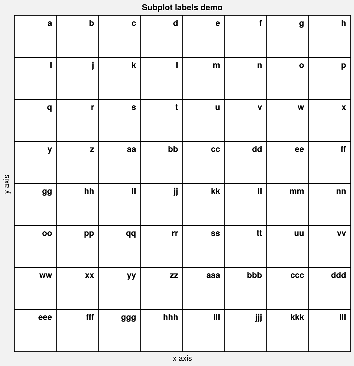
[2]:
import proplot as pplt
fig, axs = pplt.subplots(nrows=8, ncols=8, refwidth=0.7, space=0)
axs.format(
    abc=True, abcloc='ur',
    xlabel='x axis', ylabel='y axis', xticks=[], yticks=[],
    suptitle='Subplot labels demo'
)
Automatic sizing
By default, ProPlot determines the suitable figure size given the geometry of your subplot grid and the size of a “reference” subplot. ProPlot can also determine the suitable figure height given a fixed figure width, and figure width given a fixed figure height.
This algorithm is controlled by
the following subplots keyword arguments:
refsets the reference subplot number (default is1, i.e. the subplot in the upper left corner).refaspectsets the reference subplot aspect ratio (default is1). You can also use the built-in matplotlibset_aspectmethod.refwidthandrefheightset the physical dimensions of the reference subplot (default isrefwidth=2). If one is specified, the other is calculated to satisfyrefaspect. If both are specified,refaspectis ignored. The dimensions of the figure are determined automatically.figwidthandfigheightset the physical dimensions of the figure. If one is specified, the other is calculated to satisfyrefaspectand the subplot spacing. If both are specified (or if the matplotlibfigsizeparameter is specified),refaspectis ignored.journalconstrains the physical dimensions of the figure so it meets requirements for submission to an academic journal. For example, figures created withjournal='nat1'are sized as single-column Nature figures. See this table for the list of available journal specifications (feel free to add to this table by submitting a PR).
The below examples demonstrate the default behavior of the figure sizing algorithm,
and how it can be controlled with subplots keyword arguments.
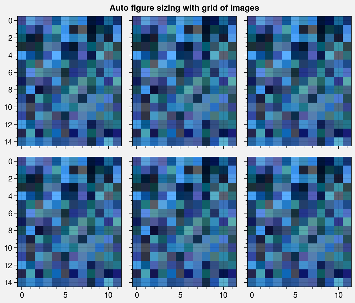
Important
The automatic figure size algorithm has the following notable properties:
For very simple subplot grids (i.e. subplots created with the
ncolsandnrowsarguments), the argumentsrefaspect,refwidth, andrefheightapply to every subplot in the figure – not just the reference subplot.When the reference subplot aspect ratio has been fixed (e.g., using
ax.set_aspect(1)) or is set to'equal'(as with geographic projections andimshowimages), the fixed aspect ratio is used and thesubplotsrefaspectparameter is ignored. This is critical for getting the figure size right when working with grids of images and grids of projections.When
colorbars andpanels are present in the figure, their physical widths are preserved during figure resizing. ProPlot specifies their widths in physical units to help avoid colorbars that look “too skinny” or “too fat”.
[3]:
import proplot as pplt
import numpy as np

# # Auto sized grid of cartopy projections
# fig, axs = pplt.subplots(ncols=2, nrows=3, proj='robin')
# axs.format(
#     land=True, landcolor='k',
#     suptitle='Auto figure sizing with grid of cartopy projections'
# )

# Auto sized grid of images
state = np.random.RandomState(51423)
fig, axs = pplt.subplots(ncols=3, nrows=2, refwidth=1.7)
colors = state.rand(15, 12, 3).cumsum(axis=2)
colors /= colors.max()
axs.imshow(colors)
axs.format(
    suptitle='Auto figure sizing with grid of images'
)
[4]:
import proplot as pplt
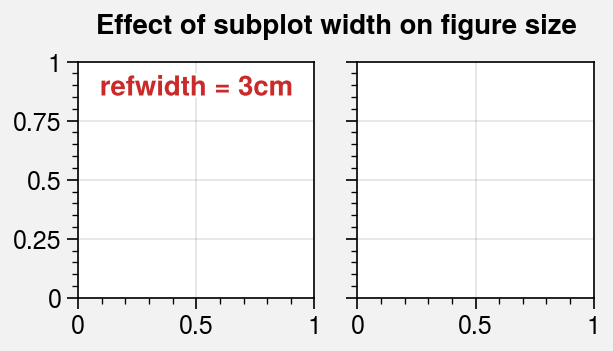
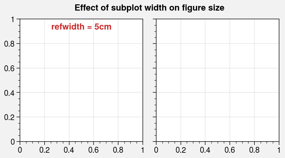
# Change the reference subplot width
suptitle = 'Effect of subplot width on figure size'
for refwidth in ('3cm', '5cm'):
fig, axs = pplt.subplots(ncols=2, refwidth=refwidth,)
axs[0].format(
suptitle=suptitle,
title=f'refwidth = {refwidth}', titleweight='bold',
titleloc='uc', titlecolor='red9',
)
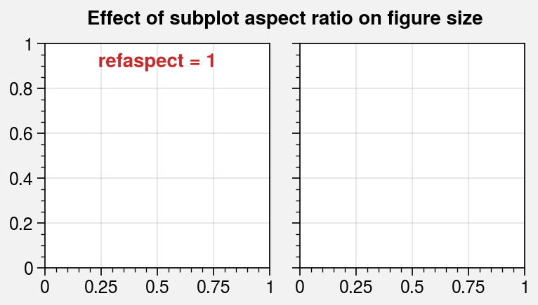
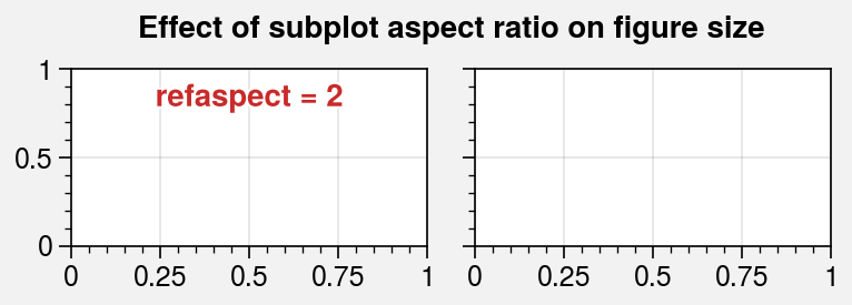
# Change the reference subplot aspect ratio
for refaspect in (1, 2):
fig, axs = pplt.subplots(ncols=2, refwidth=1.6, refaspect=refaspect)
axs[0].format(
suptitle='Effect of subplot aspect ratio on figure size',
title=f'refaspect = {refaspect}', titleweight='bold',
titleloc='uc', titlecolor='red9',
)
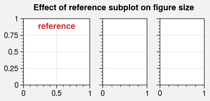
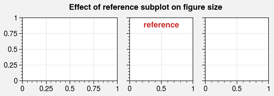
[5]:
import proplot as pplt
# Change the reference subplot in presence of unequal width/height ratios
for ref in (1, 2):
fig, axs = pplt.subplots(
ncols=3, wratios=(3, 2, 2), ref=ref, refwidth=1.1,
)
axs[ref - 1].format(
suptitle='Effect of reference subplot on figure size',
title='reference', titleweight='bold',
titleloc='uc', titlecolor='red9'
)
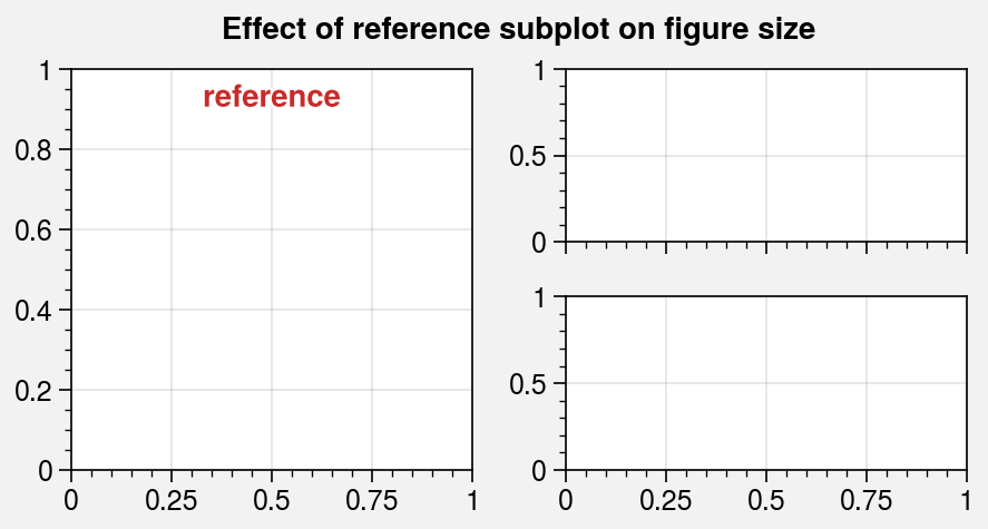
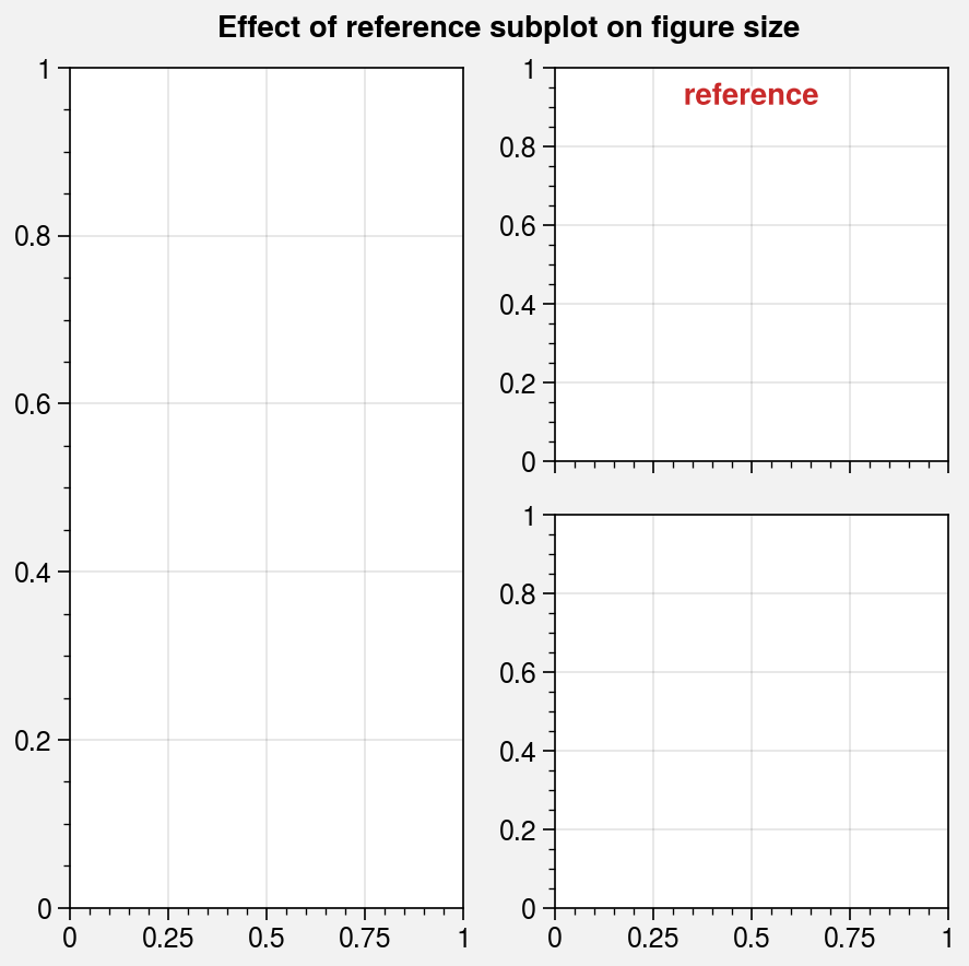
# Change the reference subplot in a complex grid
for ref in (1, 2):
fig, axs = pplt.subplots(
[[1, 2], [1, 3]],
ref=ref, refwidth=1.8, span=False
)
axs[ref - 1].format(
suptitle='Effect of reference subplot on figure size',
title='reference', titleweight='bold',
titleloc='uc', titlecolor='red9'
)
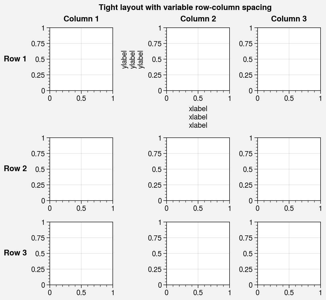
Automatic spacing
In addition to automatic figure sizing, by default ProPlot applies a tight layout
algorithm to every figure. This algorithm automatically adjusts the space between
subplot rows and columns and the figure edge to accommodate labels.
It can be disabled by passing tight=False to subplots.
While matplotlib has its own tight layout algorithm,
ProPlot’s algorithm may change the figure size to accommodate the correct spacing
and permits variable spacing between subsequent subplot rows and columns (see the
new GridSpec class for details).
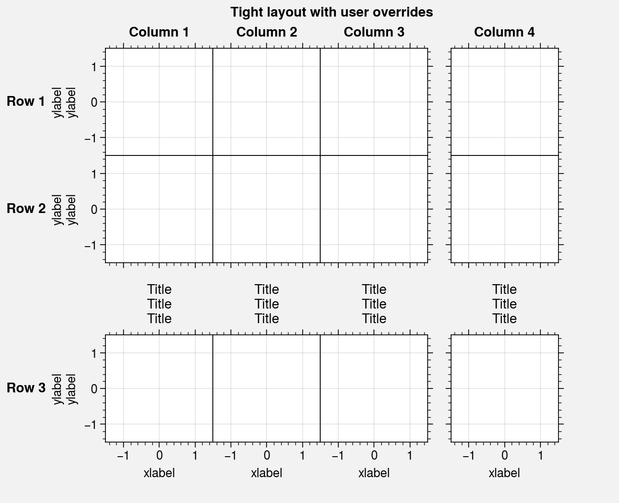
The tight layout algorithm can also be overridden. When you use any
of the spacing arguments left, right, top, bottom, wspace, or
hspace, that value is always respected. For example:
left='2em'fixes the left margin width, while the right, bottom, and top margin widths are determined automatically.wspace='1em'fixes the spaces between subplot columns, while the spaces between subplot rows are determined automatically.wspace=('3em', None)fixes the space between the first two columns of a three-column plot, while the space between the second two columns is determined automatically.
The below examples demonstrate how the tight layout algorithm permits variable spacing between subplot rows and columns.
[6]:
import proplot as pplt

# Automatic spacing for all margins and between all columns and rows
fig, axs = pplt.subplots(nrows=3, ncols=3, refwidth=1.1, share=0)

# Formatting that stress-tests the algorithm
axs[1].format(xlabel='xlabel\nxlabel\nxlabel', ylabel='ylabel\nylabel\nylabel')
axs.format(
    toplabels=('Column 1', 'Column 2', 'Column 3'),
    leftlabels=('Row 1', 'Row 2', 'Row 3'),
    suptitle='Tight layout with variable row-column spacing'
)
[7]:
import proplot as pplt

# Manual spacing for certain margins and between certain columns and rows
fig, axs = pplt.subplots(
    ncols=4, nrows=3, refwidth=1.1, span=False,
    bottom='5em', right='5em',  # margin spacing overrides
    wspace=(0, 0, None), hspace=(0, None),  # column and row spacing overrides
)

# Formatting that stress-tests the algorithm
axs.format(
    xlim=(-1.5, 1.5), ylim=(-1.5, 1.5), xlocator=1, ylocator=1,
    suptitle='Tight layout with user overrides',
    toplabels=('Column 1', 'Column 2', 'Column 3', 'Column 4'),
    leftlabels=('Row 1', 'Row 2', 'Row 3'),
)
axs[0, :].format(xtickloc='top')
axs[2, :].format(xtickloc='both')
axs[:, 1].format(ytickloc='neither')
axs[:, 2].format(ytickloc='right')
axs[:, 3].format(ytickloc='both')
axs[-1, :].format(title='Title\nTitle\nTitle', xlabel='xlabel')
axs[:, 0].format(ylabel='ylabel\nylabel')
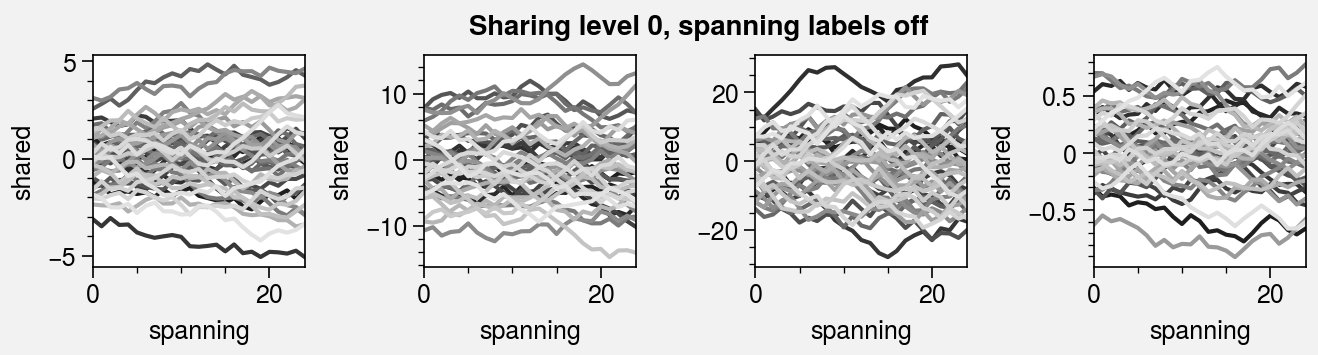
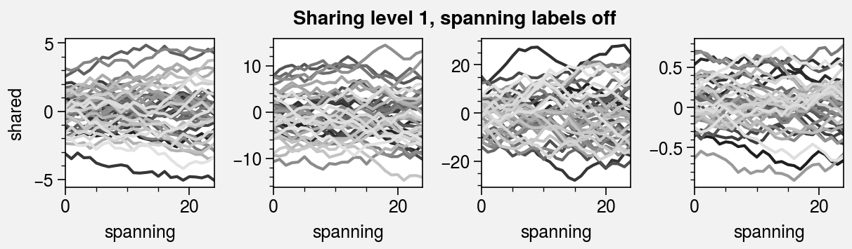
Axis sharing
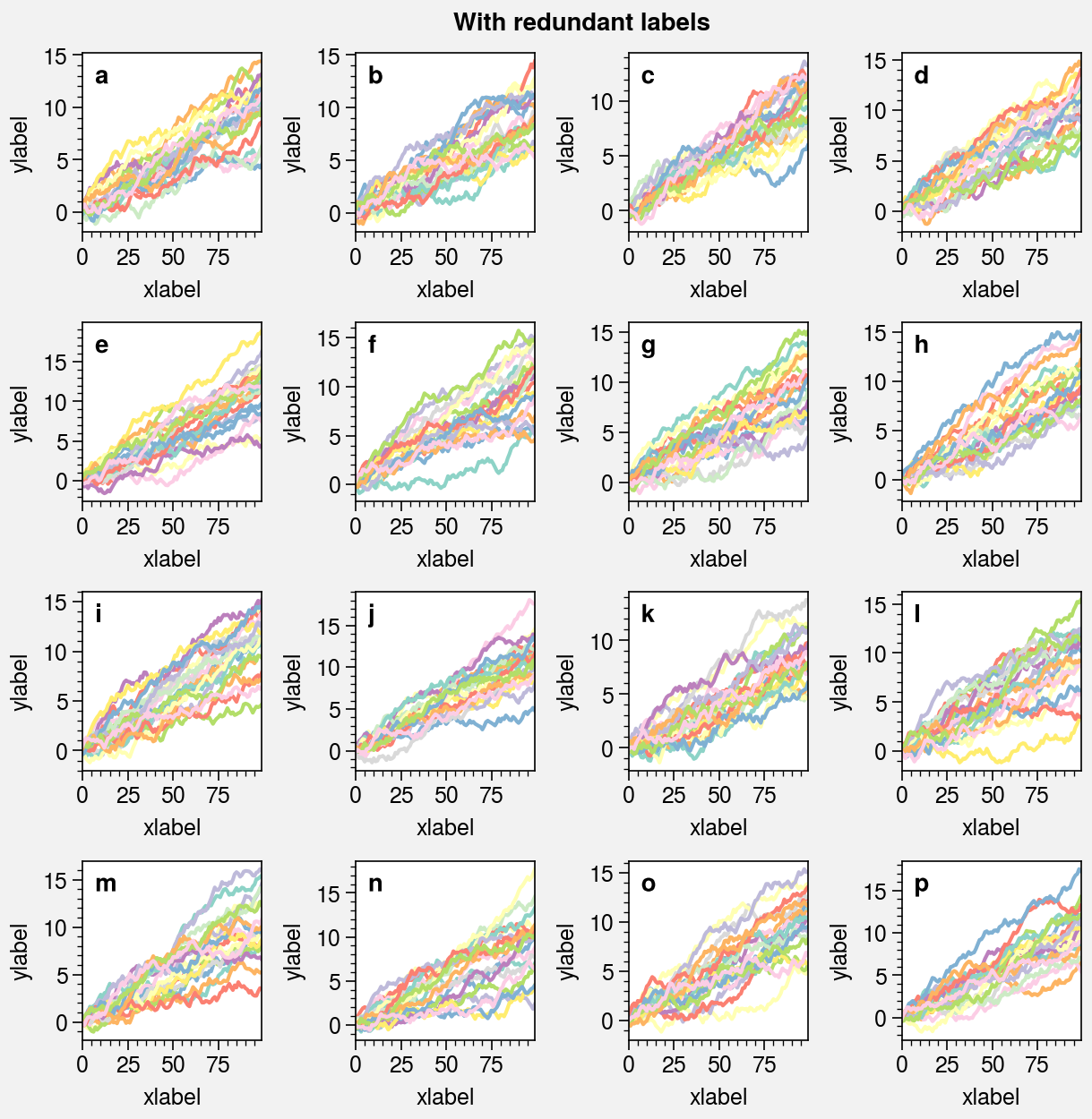
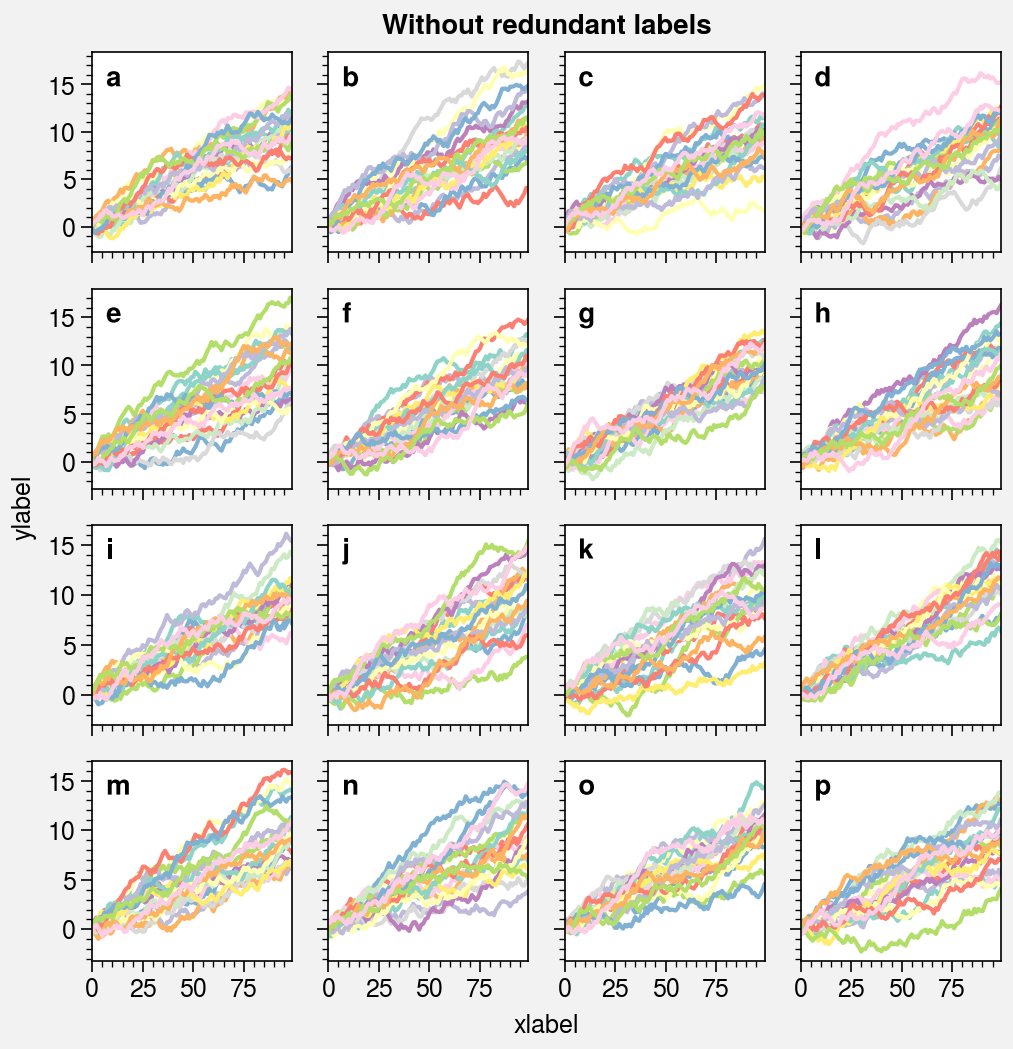
Redundant labels are a common problem for figures with lots of
subplots. To address this, matplotlib.pyplot.subplots includes the sharex and
sharey keyword arguments that permit sharing axis limits, ticks, and tick labels
between like rows and columns of subplots. ProPlot expands upon this feature by…
Adding an option for sharing labels in the same row or column of the subplot grid, controlled by the
spanxandspanykeywords (default isrc[‘subplots.span’]=True). Use thespankeyword as shorthand to set bothspanxandspany.Adding four axis-sharing “levels”, controlled by the
sharexandshareykeywords (default isrc[‘subplots.share’]=3). Use thesharekeyword as shorthand to set bothsharexandsharey. The axis-sharing “levels” are defined as follows:Level
0disables axis sharing.Level
1shares the axis labels, but nothing else.Level
2is the same as1, but the axis limits, ticks, and scales are also shared.Level
3is the same as2, but the axis tick labels are also shared.
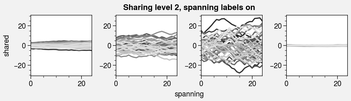
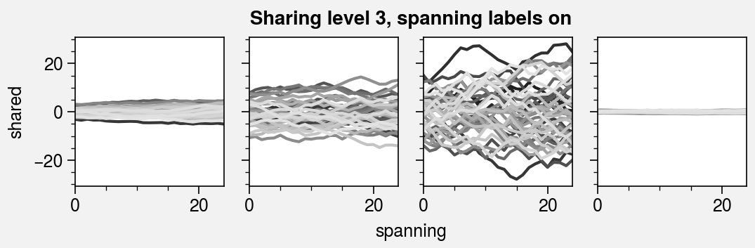
Axis and label sharing works for arbitrarily complex subplot grids. The below examples demonstrate the effect of various axis and label sharing settings on the appearance of simple subplot grids.
[8]:
import proplot as pplt
import numpy as np
N = 50
M = 40
state = np.random.RandomState(51423)
colors = pplt.Colors('grays_r', M, left=0.1, right=0.8)
datas = []
for scale in (1, 3, 7, 0.2):
    data = scale * (state.rand(N, M) - 0.5).cumsum(axis=0)[N // 2:, :]
    datas.append(data)

# Same plot with different sharing and spanning settings
for share in (0, 1, 2, 3):
    fig, axs = pplt.subplots(
        ncols=4, refaspect=1, refwidth=1.06,
        sharey=share, spanx=share // 2
    )
    for ax, data in zip(axs, datas):
        on = ['off', 'on'][share // 2]
        ax.plot(data, cycle=colors)
        ax.format(
            suptitle=f'Sharing level {share}, spanning labels {on}',
            grid=False, xlabel='spanning', ylabel='shared'
        )
[9]:
import proplot as pplt
import numpy as np
pplt.rc.reset()
pplt.rc.cycle = 'Set3'
state = np.random.RandomState(51423)
titles = ['With redundant labels', 'Without redundant labels']

# Same plot with and without default sharing settings
for mode in (0, 1):
    fig, axs = pplt.subplots(
        nrows=4, ncols=4, share=3 * mode,
        span=1 * mode, refwidth=1
    )
    for ax in axs:
        ax.plot((state.rand(100, 20) - 0.4).cumsum(axis=0))
    axs.format(
        xlabel='xlabel', ylabel='ylabel', suptitle=titles[mode],
        abc=True, abcloc='ul',
        grid=False, xticks=25, yticks=5
    )
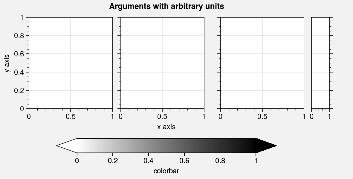
Physical units
ProPlot supports arbitrary physical units for controlling the figure
figwidth and figheight, the reference subplot refwidth and refheight,
the gridspec spacing values left, right, bottom, top, wspace, and
hspace, and in a few other places, e.g. panel and
colorbar widths. This feature is powered by the
units function.
If a sizing argument is numeric, the units are inches or points; if it is
string, the units are converted to inches or points by
units. A table of acceptable units is found in the
units documentation. They include centimeters,
millimeters, pixels,
em-heights,
en-heights,
and points.
[10]:
import proplot as pplt
import numpy as np
with pplt.rc.context(fontsize='12px'):
    fig, axs = pplt.subplots(
        ncols=3, figwidth='15cm', figheight='3in',
        wspace=('10pt', '20pt'), right='10mm'
    )
    cmap = pplt.Colormap('Mono')
    cb = fig.colorbar(
        cmap, loc='b', extend='both', label='colorbar',
        width='2em', extendsize='3em', shrink=0.8,
    )
    pax = axs[2].panel('r', width='5en')
    pax.format(xlim=(0, 1))
axs.format(
    suptitle='Arguments with arbitrary units',
    xlabel='x axis', ylabel='y axis',
    xlim=(0, 1), ylim=(0, 1),
)