Geographic and polar plots
ProPlot includes features for working with polar axes and the cartopy and basemap geographic projection packages. These features are optional. Installation of cartopy or basemap is not required.
To change the axes projection, pass proj='name' to subplots. To use
different projections for different subplots, pass a dictionary of projection names
with the subplot number as the key – for example, proj={1: 'name'}. The default
projection is always CartesianAxes (it can be explicitly specified
with proj='cartesian').
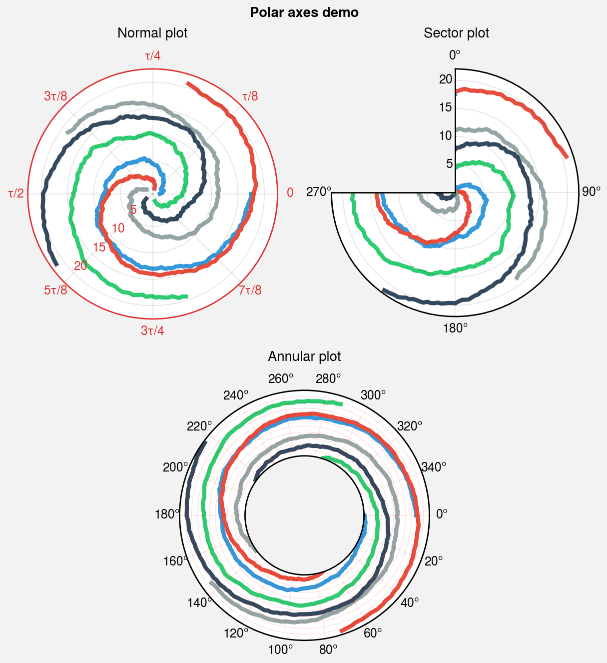
Polar axes
To draw polar axes, pass proj='polar' or e.g. proj={1: 'polar'}
to subplots. This generates a proplot.axes.PolarAxes instance with
its own format method.
The proplot.axes.PolarAxes.format method facilitates polar-specific axes
modifications like changing the central radius r0, the zero azimuth location
theta0, and the positive azimuthal direction thetadir. It also supports
changing gridline locations with rlocator and thetalocator (analogous to
ylocator and xlocator used by format) and
turning your polar plot into an “annular” or “sector” plot by changing the radial
limits rlim or the azimuthal limits thetalim. Finally, since
proplot.axes.PolarAxes.format calls proplot.axes.Axes.format, it can be used to
add axes titles, a-b-c labels, and figure titles, just like
CartesianAxes.
For details, see proplot.axes.PolarAxes.format.
[1]:
import proplot as pplt
import numpy as np
N = 200
state = np.random.RandomState(51423)
x = np.linspace(0, 2 * np.pi, N)
y = 100 * (state.rand(N, 5) - 0.3).cumsum(axis=0) / N
fig, axs = pplt.subplots([[1, 1, 2, 2], [0, 3, 3, 0]], proj='polar')
axs.format(
    suptitle='Polar axes demo', linewidth=1, titlepad='1em',
    ticklabelsize=9, rlines=0.5, rlim=(0, 19),
)
for i in range(5):
    xi = x + i * 2 * np.pi / 5
    axs.plot(xi, y[:, i], cycle='FlatUI', zorder=0, lw=3)

# Standard polar plot
axs[0].format(
    title='Normal plot', thetaformatter='tau',
    rlabelpos=225, rlines=pplt.arange(5, 30, 5),
    color='red8', tickpad='1em',
)

# Sector plot
axs[1].format(
    title='Sector plot', thetadir=-1, thetalines=90, thetalim=(0, 270), theta0='N',
    rlim=(0, 22), rlines=pplt.arange(5, 30, 5),
)

# Annular plot
axs[2].format(
    title='Annular plot', thetadir=-1, thetalines=20, gridcolor='red',
    r0=-20, rlim=(0, 22), rformatter='null', rlocator=2
)
Geographic axes
ProPlot can create geographic projection axes using
either cartopy or basemap as “backends”. To draw geographic axes, pass
proj='name' or e.g. proj={2: 'name'} (see above) to
subplots where name is any valid PROJ projection name. You can also use proj=projection_instance, where
projection_instance is a cartopy.crs.Projection or
mpl_toolkits.basemap.Basemap returned by the Proj
constructor function.
When you request a geographic projection, subplots returns
a proplot.axes.GeoAxes instance with its own format
method. The proplot.axes.GeoAxes.format method lets you
modify geographic features with the same syntax for
either backend. A few details:
Cartopy is the default backend. When you request projections with cartopy as the backend,
subplotsreturnsproplot.axes.CartopyAxes, which is a subclass of bothproplot.axes.GeoAxesandcartopy.mpl.geoaxes.GeoAxes. Under the hood, invokingformaton aCartopyAxeschanges map bounds usingset_extent, adds major and minor gridlines usinggridlines, and adds geographic features usingadd_feature. If you prefer, you can use the standardcartopy.mpl.geoaxes.GeoAxesmethods just like you would in cartopy.Basemap is an alternative backend. To use basemap, set
rc.basemaptoTrueor passbasemap=Truetosubplots. When you request projections with basemap as the backend,subplotsreturnsproplot.axes.BasemapAxes, which is a subclass ofproplot.axes.GeoAxes.BasemapAxesredirects the plot, scatter, contour, contourf, pcolor, pcolormesh, quiver, streamplot, and barb methods to identically named methods on theBasemapinstance. This means you can work with the standard axes plotting methods rather than the basemap methods – just like cartopy. Under the hood, invokingformaton aBasemapAxesadds major and minor gridlines usingdrawmeridiansanddrawparallelsand adds geographic features using methods likefillcontinentsanddrawcoastlines. If you need to use the underlyingBasemapinstance, it is available via theproplot.axes.BasemapAxes.projectionattribute.
Together, these features let you work with geophysical data without invoking
verbose cartopy classes like LambertAzimuthalEqualArea and
NaturalEarthFeature or keeping track of separate
Basemap instances. They considerably reduce the amount of
code needed to make geographic plots. In the below examples, we create a variety
of geographic plots using both cartopy and basemap as backends.
Note
By default, ProPlot gives circular boundaries to polar cartopy projections like
NorthPolarStereo(see this example from the cartopy website). This is consistent with basemap’s default behavior. To disable this feature, setrc[‘cartopy.circular’]toFalse. Please note that cartopy cannot add gridline labels to polar plots with circular boundaries.By default, ProPlot uses
set_globalto give non-polar cartopy projections global extent and bounds polar cartopy projections at the equator. This is a deviation from cartopy, which determines map boundaries automatically based on the coordinates of the plotted content. To revert to cartopy’s default behavior, setrc[‘cartopy.autoextent’]toTrue.To make things more consistent between cartopy and basemap, the
Projconstructor function lets you supply native PROJ keyword names for the cartopyProjectionclasses (e.g.,lon_0instead ofcentral_longitude) and instantiatesBasemapprojections with sensible default PROJ parameters rather than raising an error when they are omitted (e.g.,lon_0=0as the default for most projections).
Warning
Basemap is no longer maintained and will not work with matplotlib versions more recent than 3.2.2. However, as shown below, gridline labels tend to look nicer in basemap than in cartopy – especially when “inline” cartopy labels are disabled. This is the main reason ProPlot continues to support both basemap and cartopy. When cartopy’s gridline labels improve, basemap support may be deprecated.
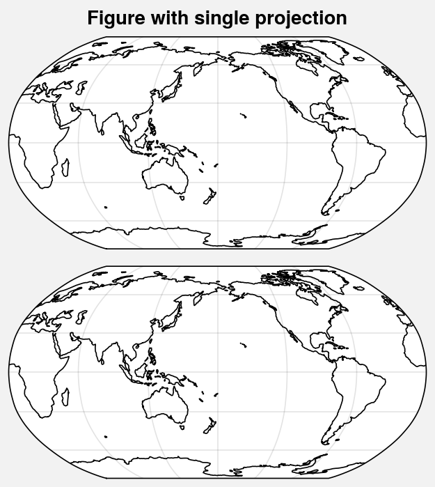
[2]:
# Simple figure with just one projection

# Option 1: Create a projection manually with pplt.Proj()
# immport proplot as plot
# proj = pplt.Proj('robin', lon_0=180)
# fig, axs = pplt.subplots(nrows=2, refwidth=3, proj=proj)

# Option 2: Pass the name to 'proj' and keyword arguments to 'proj_kw'
import proplot as pplt
fig, axs = pplt.subplots(nrows=2, refwidth=3, proj='robin', proj_kw={'lon_0': 180})
axs.format(
    suptitle='Figure with single projection',
    coast=True, latlines=30, lonlines=60,
)
/home/docs/checkouts/readthedocs.org/user_builds/proplot/conda/v0.7.0/lib/python3.8/site-packages/cartopy/io/__init__.py:260: DownloadWarning: Downloading: https://naciscdn.org/naturalearth/110m/physical/ne_110m_coastline.zip
  warnings.warn('Downloading: {}'.format(url), DownloadWarning)
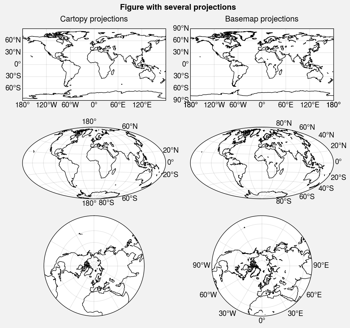
[3]:
# Complex figure with different projections
import proplot as pplt
fig, axs = pplt.subplots(
    ncols=2, nrows=3,
    hratios=(1, 1, 1.4),
    basemap=(False, True, False, True, False, True),  # cartopy column 1
    proj=('cyl', 'cyl', 'hammer', 'hammer', 'npstere', 'npstere'),
)
axs.format(
    suptitle='Figure with several projections',
    toplabels=('Cartopy projections', 'Basemap projections'),
    toplabelweight='normal',
    coast=True, latlines=20, lonlines=30,
    lonlabels='b', latlabels='r',  # or lonlabels=True, labels=True, etc.
)
axs[0, :].format(latlines=30, lonlines=60, labels=True)
pplt.rc.reset()
Warning: Cannot label meridians on Hammer basemap
Geographic plotting
In ProPlot, plotting with GeoAxes is not much different from
plotting with CartesianAxes. ProPlot makes longitude-latitude (i.e.,
Plate Carrée) coordinates the default coordinate system by passing
transform=ccrs.PlateCarree() to cartopy plotting commands and latlon=True to
basemap plotting commands. And again, basemap plotting commands are invoked from the
proplot.axes.GeoAxes rather than the Basemap instance –
just like cartopy. When using basemap as the “backend”, you should not have to work
with the Basemap instance directly.
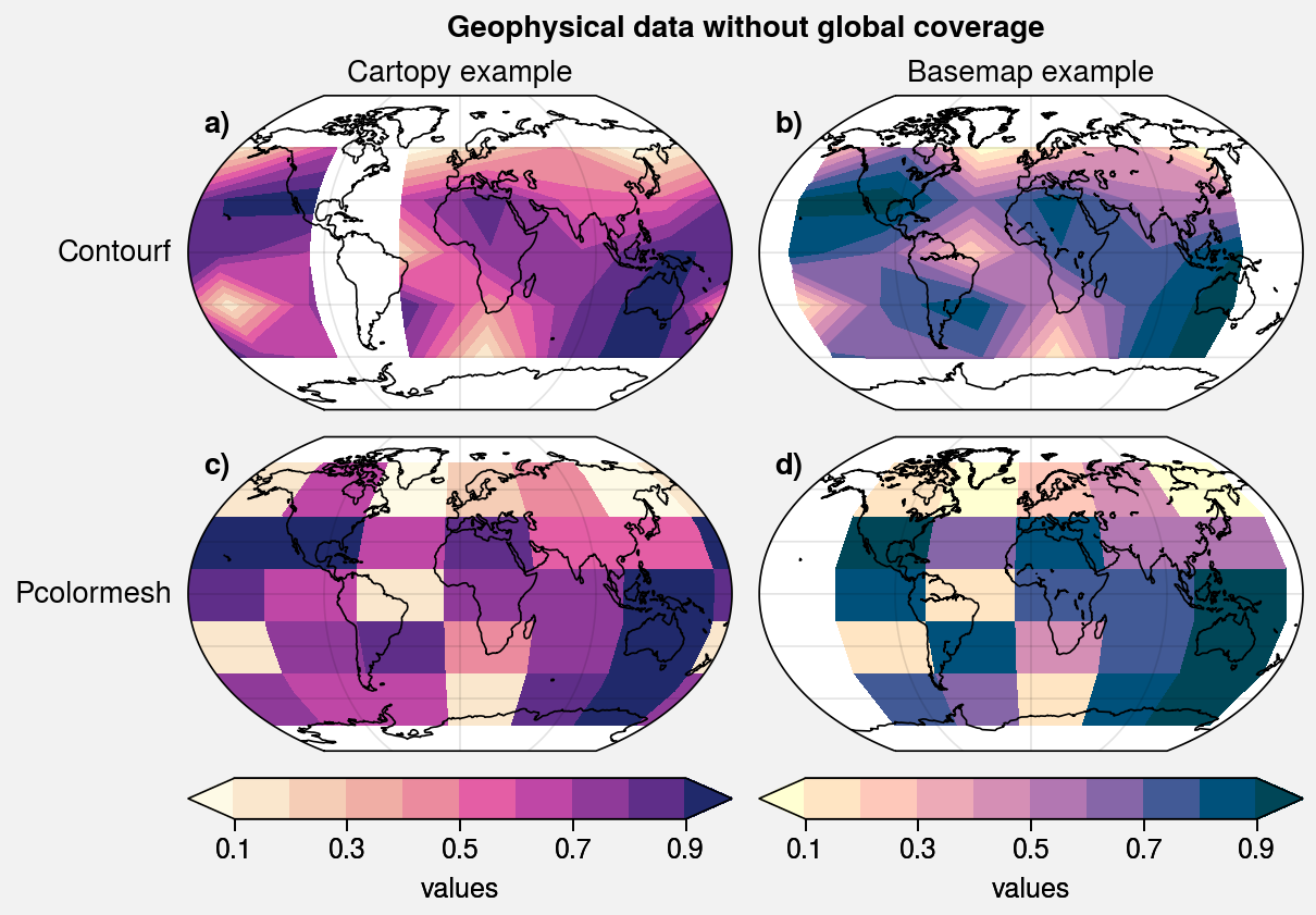
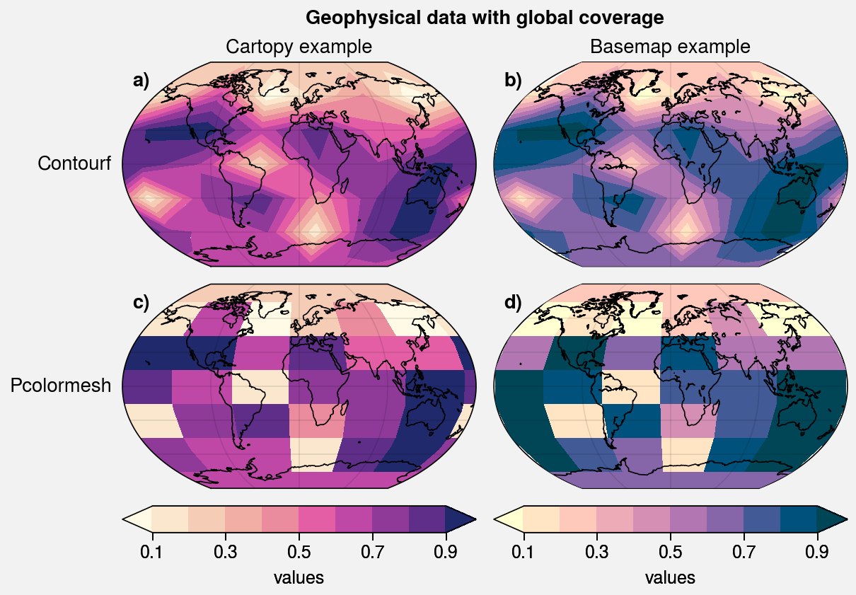
To ensure the graphics generated by 2D plotting commands like
contour fill the entire globe, simply pass globe=True to
the plotting command. This interpolates your data to the poles and across the
longitude seam before plotting the data. This is a convenient alternative to
cartopy’s add_cyclic_point and basemap’s
addcyclic.
Geographic features can be drawn underneath data or on top of data by changing the
corresponding zorder
setting. For example, to draw land patches on top of all plotted content as
a “land mask,” use ax.format(land=True, landzorder=4) or set rc[‘land.zorder’]
to True. See the next section for details.
[4]:
import proplot as pplt
import numpy as np

# Fake data with unusual longitude seam location and without coverage over poles
offset = -40
lon = pplt.arange(offset, 360 + offset - 1, 60)
lat = pplt.arange(-60, 60 + 1, 30)
state = np.random.RandomState(51423)
data = state.rand(len(lat), len(lon))

# Plot data both without and with globe=True
for globe in (False, True):
    string = 'with' if globe else 'without'
    fig, axs = pplt.subplots(
        ncols=2, nrows=2, refwidth=2.5,
        proj='kav7', basemap={(1, 3): False, (2, 4): True}
    )
    axs.format(
        suptitle=f'Geophysical data {string} global coverage',
        toplabels=('Cartopy example', 'Basemap example'),
        leftlabels=('Contourf', 'Pcolormesh'),
        toplabelweight='normal', leftlabelweight='normal',
        abc=True, abcstyle='a)', abcloc='ul', abcborder=False,
        coast=True, lonlines=90,
    )
    for i, ax in enumerate(axs):
        cmap = ('sunset', 'sunrise')[i % 2]
        if i < 2:
            m = ax.contourf(lon, lat, data, cmap=cmap, globe=globe, extend='both')
            fig.colorbar(m, loc='b', span=i + 1, label='values', extendsize='1.7em')
        else:
            ax.pcolor(lon, lat, data, cmap=cmap, globe=globe, extend='both')
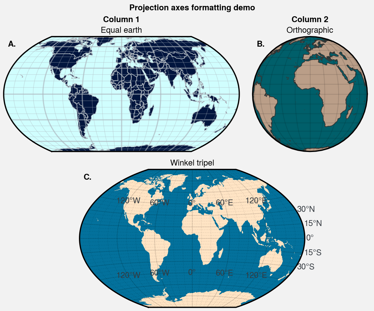
Formatting projections
The proplot.axes.GeoAxes.format method facilitates geographic-specific axes
modifications. It can be used to configure “major” and “minor” longitude and
latitude gridline locations using lonlocator, latlocator, lonminorlocator,
and latminorlocator or configure gridline label formatting with lonformatter
and latformatter (analogous to xlocator, xminorlocator, and xformatter
used by proplot.axes.CartesianAxes.format). It can also set cartopy projection
bounds with lonlim and latlim, set circular polar projection bounds with
boundinglat, and toggle and configure geographic features like land masses,
coastlines, and administrative borders using settings like
land and landcolor. Finally, since proplot.axes.GeoAxes.format
calls proplot.axes.Axes.format, it can be used to add axes titles,
a-b-c labels, and figure titles, just like CartesianAxes.
For details, see the proplot.axes.GeoAxes.format documentation.
[5]:
import proplot as pplt
fig, axs = pplt.subplots(
    [[1, 1, 2], [3, 3, 3]],
    refwidth=4, proj={1: 'eqearth', 2: 'ortho', 3: 'wintri'},
    wratios=(1, 1, 1.2), hratios=(1, 1.2),
)
axs.format(
    suptitle='Projection axes formatting demo',
    toplabels=('Column 1', 'Column 2'),
    abc=True, abcstyle='A.', abcloc='ul', abcborder=False, linewidth=1.5
)

# Styling projections in different ways
ax = axs[0]
ax.format(
    title='Equal earth', land=True, landcolor='navy', facecolor='pale blue',
    coastcolor='gray5', borderscolor='gray5', innerborderscolor='gray5',
    gridlinewidth=1.5, gridcolor='gray5', gridalpha=0.5,
    gridminor=True, gridminorlinewidth=0.5,
    coast=True, borders=True, borderslinewidth=0.8,
)
ax = axs[1]
ax.format(
    title='Orthographic', reso='med', land=True, coast=True, latlines=10, lonlines=15,
    landcolor='mushroom', suptitle='Projection axes formatting demo',
    facecolor='petrol', coastcolor='charcoal', coastlinewidth=0.8, gridlinewidth=1
)
ax = axs[2]
ax.format(
    land=True, facecolor='ocean blue', landcolor='bisque', title='Winkel tripel',
    lonlines=60, latlines=15,
    gridlinewidth=0.8, gridminor=True, gridminorlinestyle=':',
    lonlabels=True, latlabels='r', loninline=True,
    gridlabelcolor='gray8', gridlabelsize='med-large',
)
/home/docs/checkouts/readthedocs.org/user_builds/proplot/conda/v0.7.0/lib/python3.8/site-packages/cartopy/io/__init__.py:260: DownloadWarning: Downloading: https://naciscdn.org/naturalearth/110m/physical/ne_110m_land.zip
  warnings.warn('Downloading: {}'.format(url), DownloadWarning)
/home/docs/checkouts/readthedocs.org/user_builds/proplot/conda/v0.7.0/lib/python3.8/site-packages/cartopy/io/__init__.py:260: DownloadWarning: Downloading: https://naciscdn.org/naturalearth/110m/cultural/ne_110m_admin_0_boundary_lines_land.zip
  warnings.warn('Downloading: {}'.format(url), DownloadWarning)
/home/docs/checkouts/readthedocs.org/user_builds/proplot/conda/v0.7.0/lib/python3.8/site-packages/cartopy/io/__init__.py:260: DownloadWarning: Downloading: https://naciscdn.org/naturalearth/50m/physical/ne_50m_land.zip
  warnings.warn('Downloading: {}'.format(url), DownloadWarning)
/home/docs/checkouts/readthedocs.org/user_builds/proplot/conda/v0.7.0/lib/python3.8/site-packages/cartopy/io/__init__.py:260: DownloadWarning: Downloading: https://naciscdn.org/naturalearth/50m/physical/ne_50m_coastline.zip
  warnings.warn('Downloading: {}'.format(url), DownloadWarning)
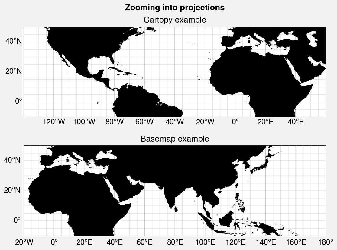
Zooming into projections
To zoom into cartopy projections, use
set_extent or pass lonlim,
latlim, or boundinglat to format. The boundinglat
keyword controls the circular latitude boundary for North Polar and
South Polar Stereographic, Azimuthal Equidistant, Lambert Azimuthal
Equal-Area, and Gnomonic projections. By default, ProPlot tries to use the
degree-minute-second cartopy locators and formatters made available in cartopy
0.18. You can switch from minute-second subintervals to traditional decimal
subintervals by passing dms=False to format
or by setting rc[‘grid.dmslabels’] to False.
To zoom into basemap projections, pass any of the boundinglat,
llcrnrlon, llcrnrlat, urcrnrlon, urcrnrlat, llcrnrx, llcrnry,
urcrnrx, urcrnry, width, or height keyword arguments to
the Proj constructor function either directly or via
the proj_kw subplots keyword argument. You can also pass
lonlim and latlim to Proj and these arguments
will be used for llcrnrlon, llcrnrlat, etc. You cannot zoom into basemap
projections with format after they have already been created.
[6]:
import proplot as pplt

# Plate Carrée map projection
pplt.rc.reso = 'med'  # use higher res for zoomed in geographic features
proj = pplt.Proj('cyl', lonlim=(-20, 180), latlim=(-10, 50), basemap=True)
fig, axs = pplt.subplots(nrows=2, refwidth=5, proj=('cyl', proj))
axs.format(
    land=True, labels=True, lonlines=20, latlines=20,
    gridminor=True, suptitle='Zooming into projections'
)
axs[0].format(
    lonlim=(-140, 60), latlim=(-10, 50),
    labels=True, title='Cartopy example'
)
axs[1].format(title='Basemap example')
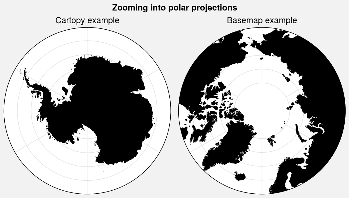
[7]:
import proplot as pplt

# Pole-centered map projections
proj = pplt.Proj('npaeqd', boundinglat=60, basemap=True)
fig, axs = pplt.subplots(ncols=2, refwidth=2.7, proj=('splaea', proj))
axs.format(
    land=True, latmax=80,  # no gridlines poleward of 80 degrees
    suptitle='Zooming into polar projections'
)
axs[0].format(boundinglat=-60, title='Cartopy example')
axs[1].format(title='Basemap example')
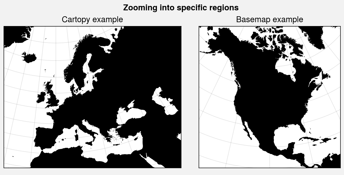
[8]:
import proplot as pplt

# Zooming in on continents
proj1 = pplt.Proj('lcc', lon_0=0)  # cartopy projection
proj2 = pplt.Proj('lcc', lon_0=-100, lat_0=45, width=8e6, height=8e6, basemap=True)
fig, axs = pplt.subplots(ncols=2, refwidth=3, proj=(proj1, proj2))
axs.format(suptitle='Zooming into specific regions', land=True)
axs[0].format(lonlim=(-20, 50), latlim=(30, 70), title='Cartopy example')
axs[1].format(lonlines=20, title='Basemap example')
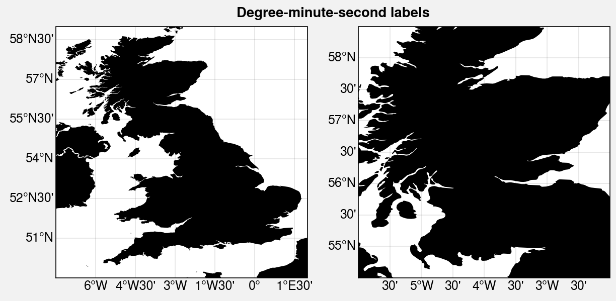
[9]:
import proplot as pplt

# Zooming to very small scale with degree-minute-second labels
pplt.rc.reso = 'hi'
fig, axs = pplt.subplots(ncols=2, refwidth=2.5, proj='cyl')
axs.format(
    land=True, labels=True,
    borders=True, borderscolor='white',
    suptitle='Degree-minute-second labels',
)
axs[0].format(lonlim=(-7.5, 2), latlim=(49.5, 59))
axs[1].format(lonlim=(-6, -2), latlim=(54.5, 58.5))
pplt.rc.reset()
/home/docs/checkouts/readthedocs.org/user_builds/proplot/conda/v0.7.0/lib/python3.8/site-packages/cartopy/io/__init__.py:260: DownloadWarning: Downloading: https://naciscdn.org/naturalearth/10m/physical/ne_10m_land.zip
  warnings.warn('Downloading: {}'.format(url), DownloadWarning)
/home/docs/checkouts/readthedocs.org/user_builds/proplot/conda/v0.7.0/lib/python3.8/site-packages/cartopy/io/__init__.py:260: DownloadWarning: Downloading: https://naciscdn.org/naturalearth/10m/cultural/ne_10m_admin_0_boundary_lines_land.zip
  warnings.warn('Downloading: {}'.format(url), DownloadWarning)
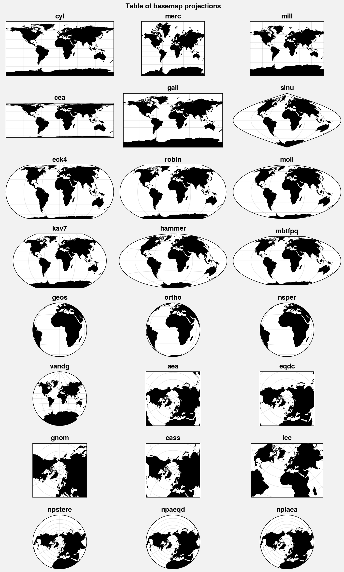
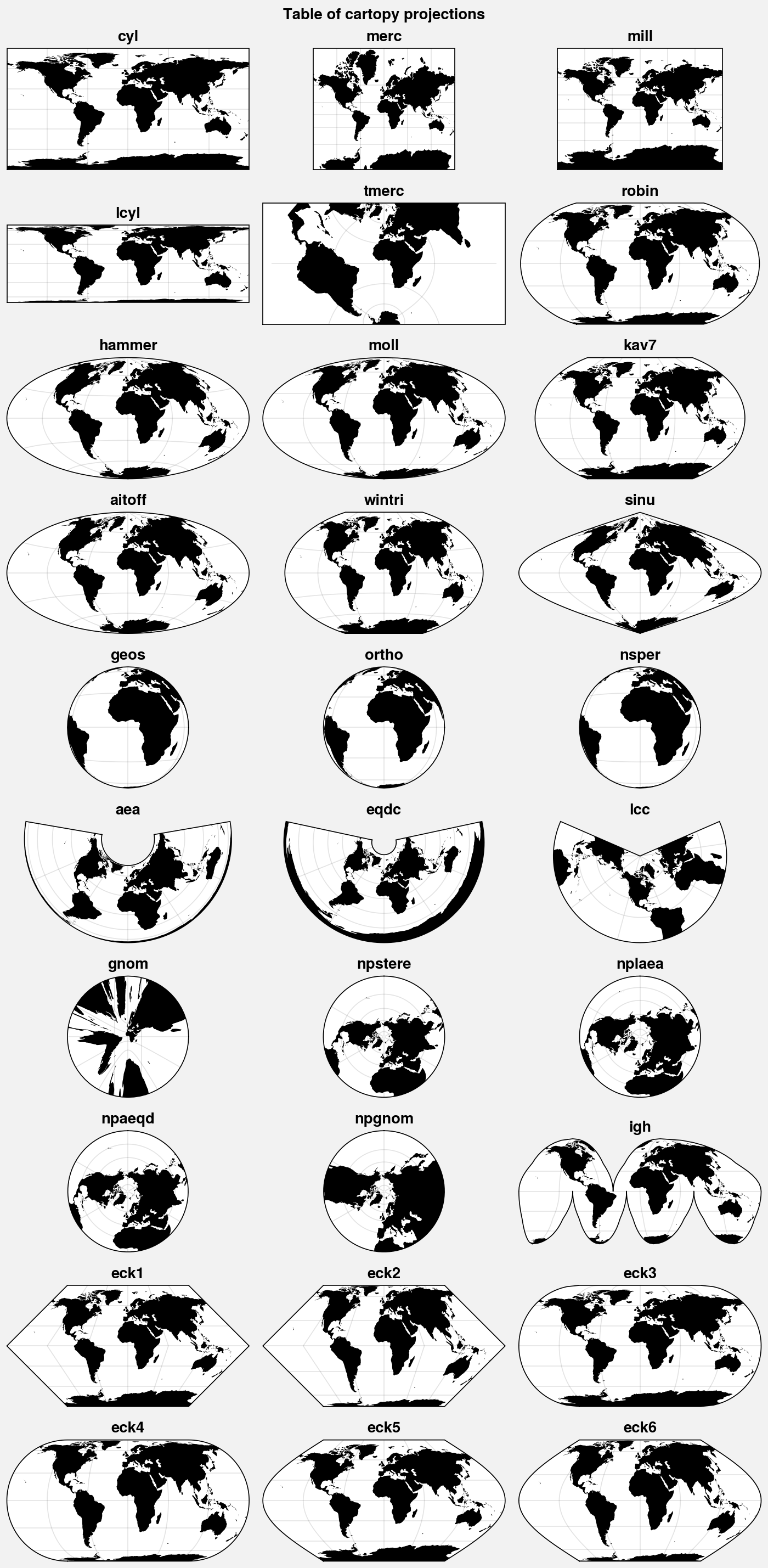
Included projections
The available cartopy
and basemap projections are
plotted below. See Proj for a table of projection
names with links to the relevant PROJ documentation.
ProPlot uses the cartopy API to add the Aitoff, Hammer, Winkel Tripel, and
Kavrisky VII projections (i.e., 'aitoff', 'hammer', 'wintri',
and 'kav7'), as well as North and South polar versions of the Azimuthal
Equidistant, Lambert Azimuthal Equal-Area, and Gnomic projections (i.e.,
'npaeqd', 'spaeqd', 'nplaea', 'splaea', 'npgnom', and
'spgnom'), modeled after the existing NorthPolarStereo
and SouthPolarStereo projections.
[10]:
import proplot as pplt

# Table of cartopy projections
projs = [
    'cyl', 'merc', 'mill', 'lcyl', 'tmerc',
    'robin', 'hammer', 'moll', 'kav7', 'aitoff', 'wintri', 'sinu',
    'geos', 'ortho', 'nsper', 'aea', 'eqdc', 'lcc', 'gnom',
    'npstere', 'nplaea', 'npaeqd', 'npgnom', 'igh',
    'eck1', 'eck2', 'eck3', 'eck4', 'eck5', 'eck6'
]
fig, axs = pplt.subplots(ncols=3, nrows=10, figwidth=7, proj=projs)
axs.format(
    land=True, reso='lo', labels=False,
    suptitle='Table of cartopy projections'
)
for proj, ax in zip(projs, axs):
    ax.format(title=proj, titleweight='bold', labels=False)
/home/docs/checkouts/readthedocs.org/user_builds/proplot/conda/v0.7.0/lib/python3.8/site-packages/proplot/constructor.py:1522: UserWarning: The default value for the *approx* keyword argument to TransverseMercator will change from True to False after 0.18.
  proj = crs(**kwproj)
/home/docs/checkouts/readthedocs.org/user_builds/proplot/conda/v0.7.0/lib/python3.8/site-packages/cartopy/mpl/feature_artist.py:154: UserWarning: Unable to determine extent. Defaulting to global.
  warnings.warn('Unable to determine extent. Defaulting to global.')
[11]:
import proplot as pplt

# Table of basemap projections
projs = [
    'cyl', 'merc', 'mill', 'cea', 'gall', 'sinu',
    'eck4', 'robin', 'moll', 'kav7', 'hammer', 'mbtfpq',
    'geos', 'ortho', 'nsper',
    'vandg', 'aea', 'eqdc', 'gnom', 'cass', 'lcc',
    'npstere', 'npaeqd', 'nplaea'
]
fig, axs = pplt.subplots(ncols=3, nrows=8, basemap=True, figwidth=7, proj=projs)
axs.format(
    land=True, labels=False,
    suptitle='Table of basemap projections'
)
for proj, ax in zip(projs, axs):
    ax.format(title=proj, titleweight='bold', labels=False)